SPY / QQQ losses

These paired examples estimate tail severity and clustering of single-session left-tail log losses relative to past EWMA return volatility. The instruments are SPY and QQQ ETFs, not the SPX and NDX index series.

Adjusted returns and retained zeros

The frozen Massive snapshot supplies split-adjusted daily closes and cash dividends. Because its adjusted=true close adjustment handles splits, dividend cash flows are included explicitly. Put prices and dividends on the same split-adjusted share basis, then compute:

r_t = log((C_t + D_t) / C_(t−1))
L_t = max(−r_t, 0)

D_t is the declared cash dividend attributed to its ex-dividend date, not its payment date. Positive returns remain in the sequence as zero losses. The first close is used only as a lag; it is not assigned an artificial zero return.

The retrieved history contains 2,329 closes and 2,328 returns through 2025-12-31. Older requested history was outside the connected account's entitlement; this is not a full-inception dataset. Trading sessions, including early-close sessions, are checked against the bounded exchange-calendar rules in the preparation script. Weekends and market holidays are not missing trading observations and are not padded.

EWMA volatility normalization

Use every signed return, including gains, to initialize and update the scale:

v_252 = mean(r_0², ..., r_251²)
v_t = 0.94 v_(t−1) + 0.06 r_(t−1)²,  t > 252
Y_t = L_t / sqrt(v_t)

This is a zero-mean EWMA volatility estimate: a root mean square of signed returns, not a mean of losses or a rolling demeaned standard deviation. The current return does not enter its own denominator. After 252 warmup sessions, both fits use 2,076 sessions from 2017-09-28 through 2025-12-31.

Y_t is dimensionless. A value of 3 means a one-session log loss three times the pre-session estimated volatility; it does not mean a 3% loss. EWMA reduces scale variation by construction but does not establish independence or stationarity.

SPY

Quantity	Estimate	Conditional 95% CI
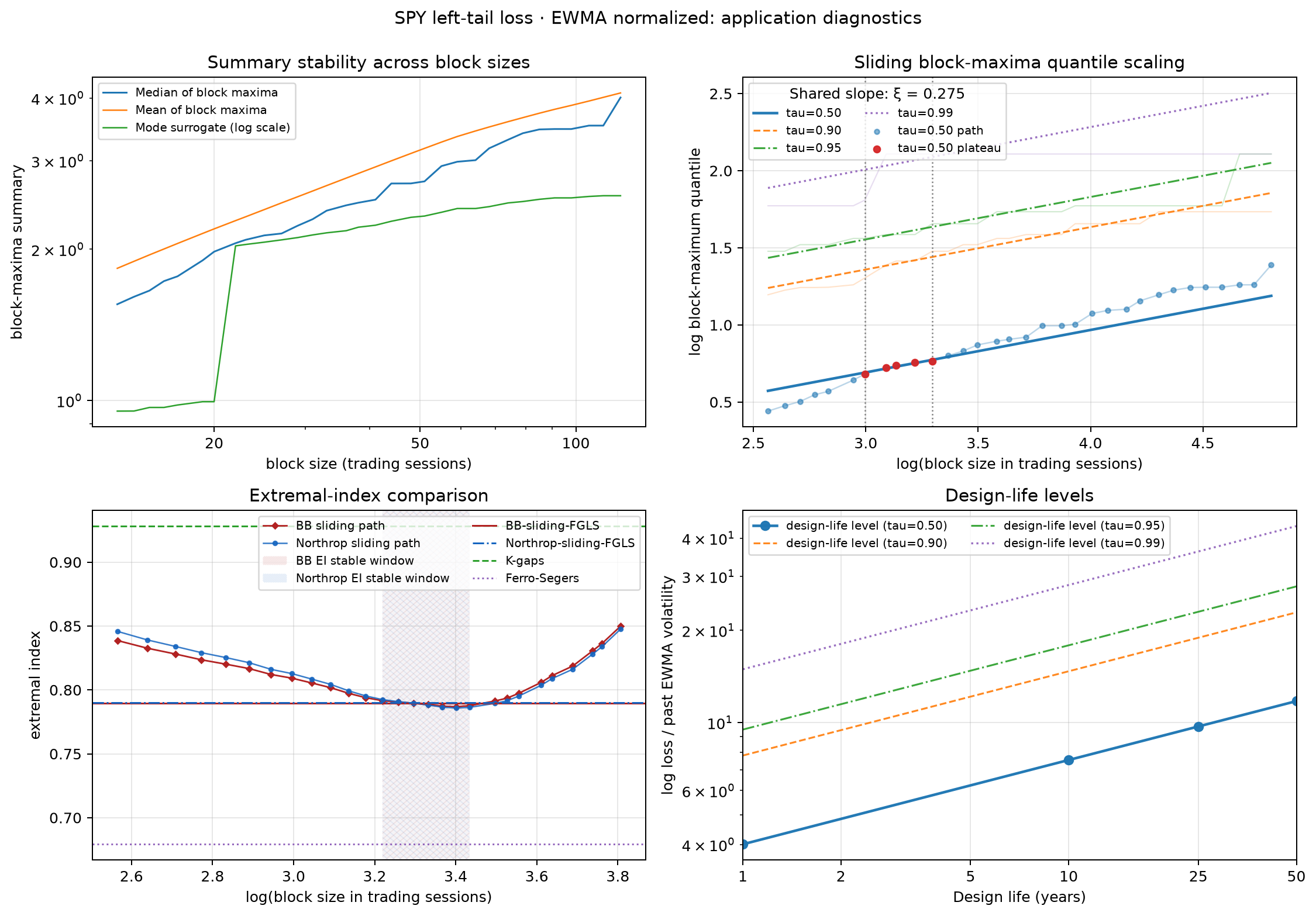
EVI ξ	0.275	[-0.230, 0.781]
BB-sliding-FGLS EI θ	0.790	[0.710, 0.879]
Northrop-sliding-FGLS EI θ	0.790	[0.710, 0.878]

All gains are retained as zero losses on the trading-session clock. Click the figure for full size.

Download numerical results and preparation settings (JSON).

The EVI window is 20–27 sessions. Its conditional interval includes zero, so this fit does not establish a positive heavy-tail index.

QQQ

Quantity	Estimate	Conditional 95% CI
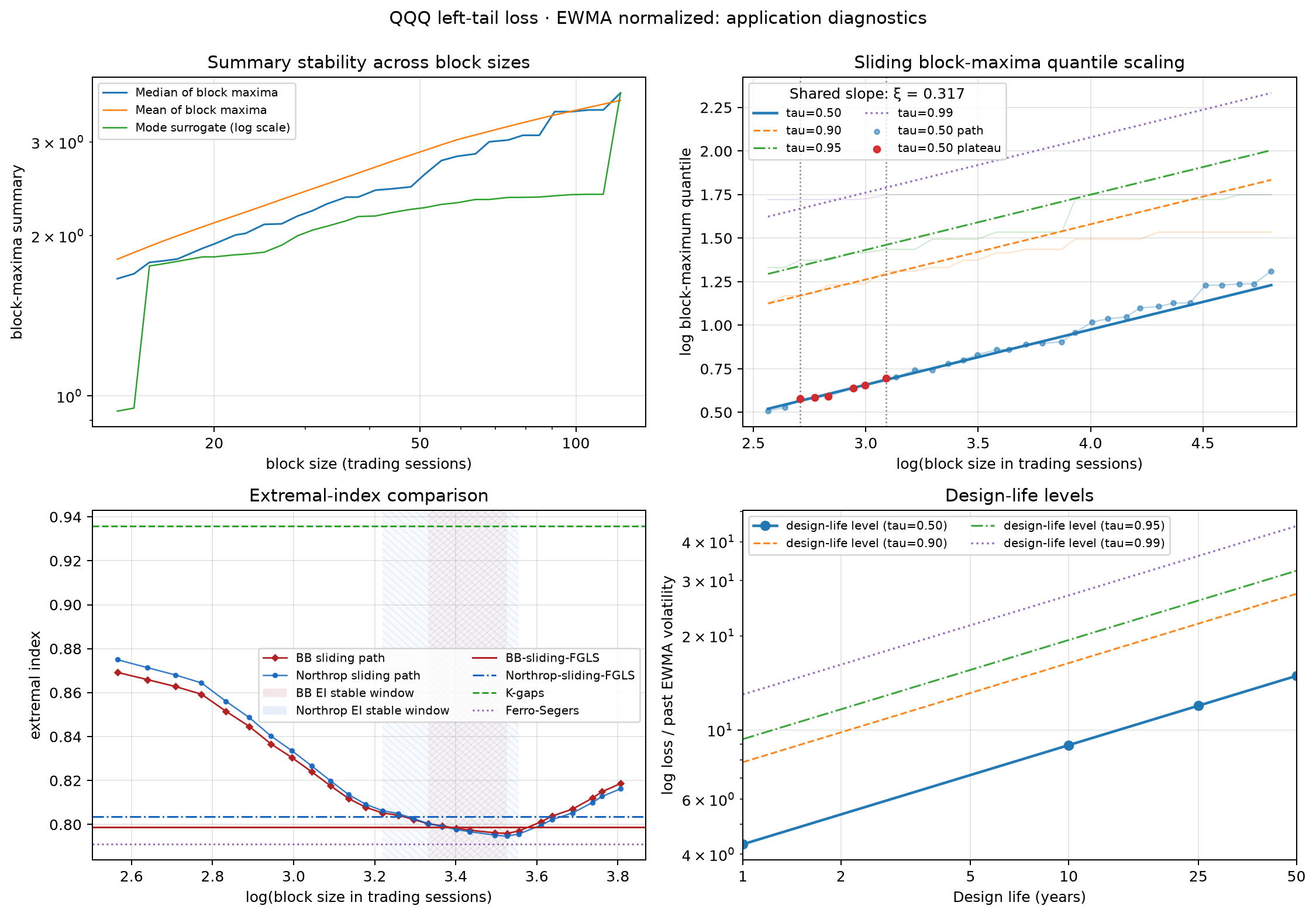
EVI ξ	0.317	[0.055, 0.579]
BB-sliding-FGLS EI θ	0.799	[0.718, 0.889]
Northrop-sliding-FGLS EI θ	0.804	[0.728, 0.888]

QQQ uses the same normalization rule and fitted dates as SPY. Click the figure for full size.

Download numerical results and preparation settings (JSON).

The EVI window is 15–22 sessions. The two EVI intervals overlap; these estimates do not establish that one ETF has a heavier tail than the other.

Interpretation and reproduction

Design-life curves use 252 trading sessions per year and target the maximum one-session normalized log loss over the horizon. They are not cumulative losses, maximum drawdowns, expected shortfall, or portfolio VaR forecasts. Long-horizon curves extrapolate far beyond the fitted block windows and the approximately eight-year normalized sample.

The nominal FGLS/Wald intervals condition on the realized normalized series; they do not refit EWMA within bootstrap draws. Historical prices and corporate actions are retrospective snapshots, not verified point-in-time vintages. These illustrations contain no strategy, transaction-cost, or trading-performance test.

To fit from local spy.csv/qqq.csv and matching provenance JSON files:

PYTHONPATH=scripts uv run python -m application.docs_cases --keys spy qqq

To reconstruct those prepared inputs from the saved Massive connector responses:

uv run python scripts/data_prep/finance_snapshot.py

The tracked script documents the split/dividend calculation and exchange-calendar checks. It reads the frozen response exports under data/raw/pilots/finance and writes inputs under data/processed/pilots; it neither requests credentials nor contacts the provider. Those responses and price histories remain local. A fresh checkout can build the documentation from the frozen figures without a provider account, but reproducing the financial fits requires the corresponding local inputs or an appropriately entitled Massive data source.