NFIP claims
The NFIP cases examine daily building-claim totals, grouped statewide by date of loss. Severity uses active days with a positive total; EI describes clustering of extreme daily totals on the calendar-day record. An active day need not be an extreme day.
Scale. “Raw” here means no EWMA normalization. Inflation adjustment to 2025 USD and aggregation by date of loss are retained. EVI uses positive claim-active days; EI uses the full calendar, including zero claim totals.
These fits use fixed shrinkage 0.73 for EVI, 0.37 for EI, and adaptive R, with unchanged claim extracts, analysis windows, and CPI inputs.
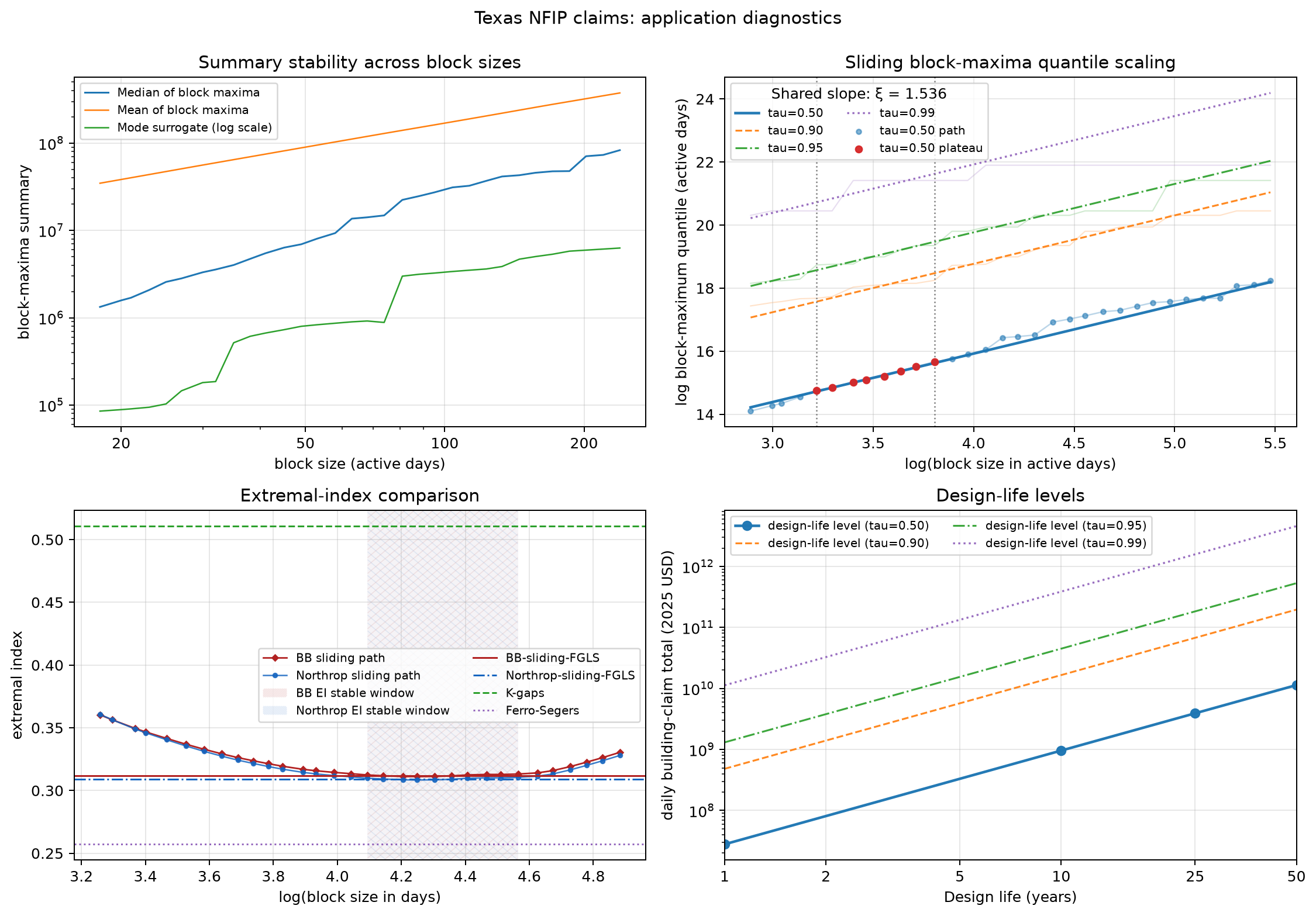
Texas daily building-claim totals
Data. OpenFEMA NFIP building-claim payments for losses dated 1978-01-01 through 2025-12-31, summed by date of loss and adjusted by loss-month CPI-U to 2025 dollars. The display and EI series contain 17,532 calendar days; the EVI series contains 5,807 positive claim-active days, or 120.979 per calendar year over the 48-year window.
For each claim, the payout multiplier is the 2025 annual-average CPI-U divided by the CPI-U for its loss month, using the not-seasonally-adjusted series. Thus all months are expressed in the same 2025-average dollar units; this is not a daily inflation adjustment or a December-2025 price base. The tracked CPI input explicitly flags October 2025 as a geometric interpolation between September and November. See the CPI input and preparation code below for that data treatment.
Download numerical results and preparation settings (JSON).
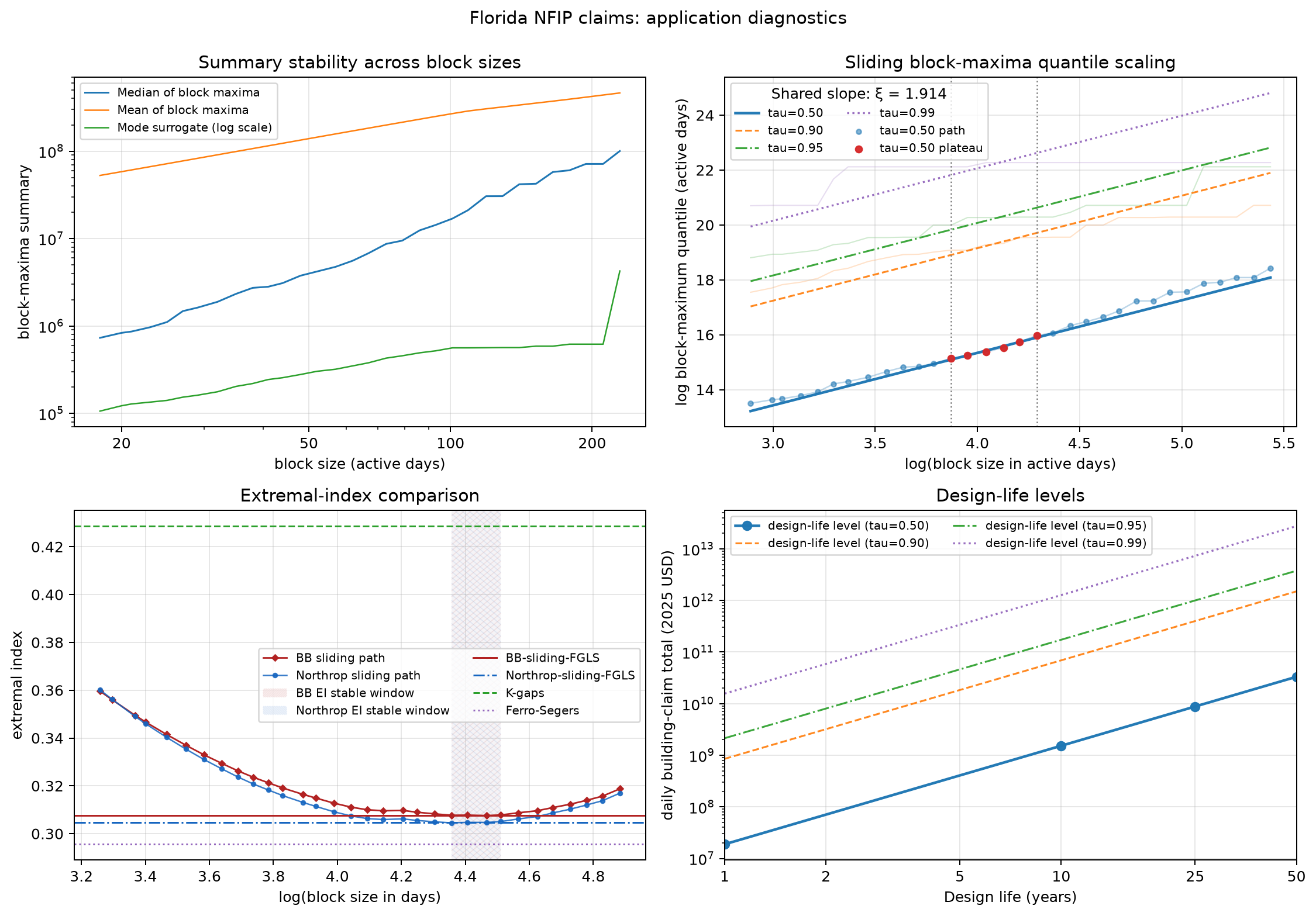
Florida daily building-claim totals
Data. The corresponding Florida series uses the same 1978-01-01 through 2025-12-31 loss-date window. It contains 17,532 calendar days and 5,440 positive claim-active days, or 113.333 per calendar year.
Download numerical results and preparation settings (JSON).
Observation clocks and design-life levels
A severity block of b observations contains b active days, which need not be
consecutive in calendar time. An EI block of size b spans b consecutive
calendar days. A zero is a zero total of recorded building-claim payments for
losses on that date.
The conversion b_T = ceil(lambda_active * T) maps a design life of T years
to a fixed number of active days, using the historical mean active-day rate.
It assumes that this rate remains applicable; variability in the future number
of active days is not modeled.
Under the stationary scaling model, the 50-year conversion gives:
| State | Active days b_50 |
Estimated median maximum daily total | Conditional 95% CI for that median |
|---|---|---|---|
| Texas | 6,049 | $11.35 billion | [$0.547, $235.46] billion |
| Florida | 5,667 | $33.17 billion | [$0.215, $5,127.40] billion |
All values are in 2025 U.S. dollars. These intervals quantify estimation
uncertainty in the median horizon maximum, D_0.5(50). They are not
prediction intervals for future maxima or the 2.5th–97.5th quantiles of those
maxima.
Why the intervals remain wide
Each severity fit uses block summaries from the full 48-year record. The selected scaling windows, however, span 25–45 active days in Texas and 48–73 in Florida. The 50-year targets of 6,049 and 5,667 active days are about 134 and 77.6 times the respective largest fitted block size. A long calendar record does not by itself validate scaling over this distance.
The interval width depends jointly on the intercept variance, slope variance, their covariance, and the target block size. Extrapolation amplifies these estimation errors, and exponentiation produces asymmetric dollar-scale bounds. At a 100-fold increase in block size, increasing the slope by 0.1 multiplies the extrapolated level by about 1.58, holding the fitted median at the reference block size fixed. Florida has the higher EVI point estimate and wider parameter uncertainty, but the parameter intervals overlap. Tail heaviness alone does not explain design-life interval width.
Further assessment should test scaling at larger block sizes and evaluate design-life interval coverage with window-selection uncertainty included. Comparable extreme-loss records and explicit modeling of changes in insured exposure and policy coverage could strengthen inference. The synthetic benchmarks evaluate EVI/EI parameter intervals; they do not establish coverage of these extrapolated design-life intervals.
Interpretation and use
The two states have similar EI point estimates. Their EVI point estimates differ, with overlapping conditional intervals. These summaries can coexist with different loss magnitudes and regional dependence structures. An asymptotic EVI above one would imply no finite mean under an unbounded regularly varying model, although fixed-probability quantiles remain finite. The reported levels describe maximum daily totals, not expected annual losses.
The curves support exploratory stress assessment across design lives and
non-exceedance probabilities. Under the fitted model and active-day-rate
conversion, tau=0.95 corresponds to a 5% probability that the maximum exceeds
the fitted level. Use in risk financing requires alignment with insured
exposure, policy terms, and event or annual loss aggregation. Totals grouped by
date of loss do not describe cash-payment timing.
CPI-U adjustment addresses inflation alone. Changes in exposure, coverage, and reporting remain outside the stationary model and its reported intervals.
- Preparation:
scripts/data_prep/fema.py - CPI treatment:
scripts/data_prep/cpi.py - Provider: OpenFEMA NFIP claims API