Benchmark

This is a statistical benchmark of estimation error and interval performance, not a runtime benchmark.

Stationary synthetic benchmarks compare severity and extremal-clustering estimates against known targets under serial dependence. The clearest gains from covariance-aware FGLS are in interval performance, with smaller changes in point accuracy.

Design and scoring

Result provenance. These results were regenerated on 2026-09-25 using the current source defaults: fixed shrinkage 0.73 for EVI and 0.37 for EI, model-based Wald intervals, and no additional CI scale calibration. The block-size grid uses lower bound max(5, ceil(n**(1/3))), EVI upper bound min(floor(n**(1 - 1/e)), floor(n/17)), and EI upper bound min(floor(sqrt(n)), floor(n/17)). Selection searches the full admissible grid without edge trimming or minimum-span expansion. EVI uses the super-block rule max(2 * B, floor(sqrt(n))) without shortening the result to increase the segment count; see Concepts. At N=365, the EVI grid has 12 levels over 8–21 and super-block length 42; the EI upper bound is 19.

The main production grid uses N=365 observations and M=100 independent simulated records per scenario, with master seed 20260401. M counts repeated datasets whose true parameter is known. R instead counts bootstrap draws within one of those datasets; increasing R does not increase M.

Branch	Process families	True parameters	Scenarios
EVI	Fréchet max-AR, moving maxima (q=99), Pareto additive AR(1)	xi = 0.01, 0.03, 0.10, 0.30, 1, 3, 10; theta = 0.01, 0.10, 0.50, 1	84
EI	Same three families	xi = 0.01, 0.50, 1, 5; theta = 0.10, 0.15, 0.25, 0.40, 0.60, 0.80, 1	84

All internal FGLS methods use the branch-specific fixed diagonal shrinkage, the declared plateau/stable-window rules, and adaptive R at 128/256/512/768/1024. The current defaults were retained after inspecting application diagnostics; this rerun on the existing simulation design is not independent validation of tuning choices. External baselines use pre-specified, method-specific tuning rules consistently across scenarios. OLS and the external estimators retain their own interval constructions.

The primary interval metric is the arithmetic mean 95% Winkler score on the parameter's original scale. For an interval [l, u] and known true value t, each score is:

W = (u - l) + 40 * max(l - t, 0) + 40 * max(t - u, 0)

Lower is better. The grid-average score is the equally weighted mean of the scenario-level means. Scores are not normalized: scenarios with larger interval widths and noncoverage penalties contribute more to this average. Scenario wins and grid-average scores therefore describe different aspects of performance. Empirical coverage complements the score by showing how often intervals contain the true parameter.

At each plotted scenario, score bars show the mean plus or minus one outer Monte Carlo standard error (MCSE), sd(W) / sqrt(n_score). These bars are not 95% confidence intervals and are not the internal MCSE used to select R. The secondary point estimation metric remains median absolute percentage error, with its 25th–75th percentile range. APE is displayed as a fraction, so 1.0 means 100% error.

Severity branch (EVI)

The EVI suite varies the true tail index, extremal dependence, and process family at a short record length. The full comparison contains 12 internal methods (three summaries, two block schemes, two regressions) and four external reference estimators. The figure shows the six core methods; the CSV outputs retain all methods, including the mean/mode and external comparisons.

Within the BM framework, median-disjoint-FGLS has the lowest grid-average Winkler score (9.261), followed by median-sliding-FGLS (9.383). Median-sliding-FGLS wins 19 of 84 scenarios and median-disjoint-FGLS wins 15. FGLS methods win 83 scenarios; mean-disjoint-OLS wins one. These rankings differ because grid-average scores retain each scenario's original parameter scale.

For median-sliding, the score is 9.383 under FGLS versus 44.707 under OLS; grid-average coverage is 79.0% versus 8.9%. FGLS improves interval performance relative to OLS here, but does not achieve nominal 95% coverage.

Six core EVI methods. Mean Winkler score uses ±1 outer MCSE; median absolute percentage error uses its IQR. Each point summarizes M=100 records in one scenario. Click the figure for full size.

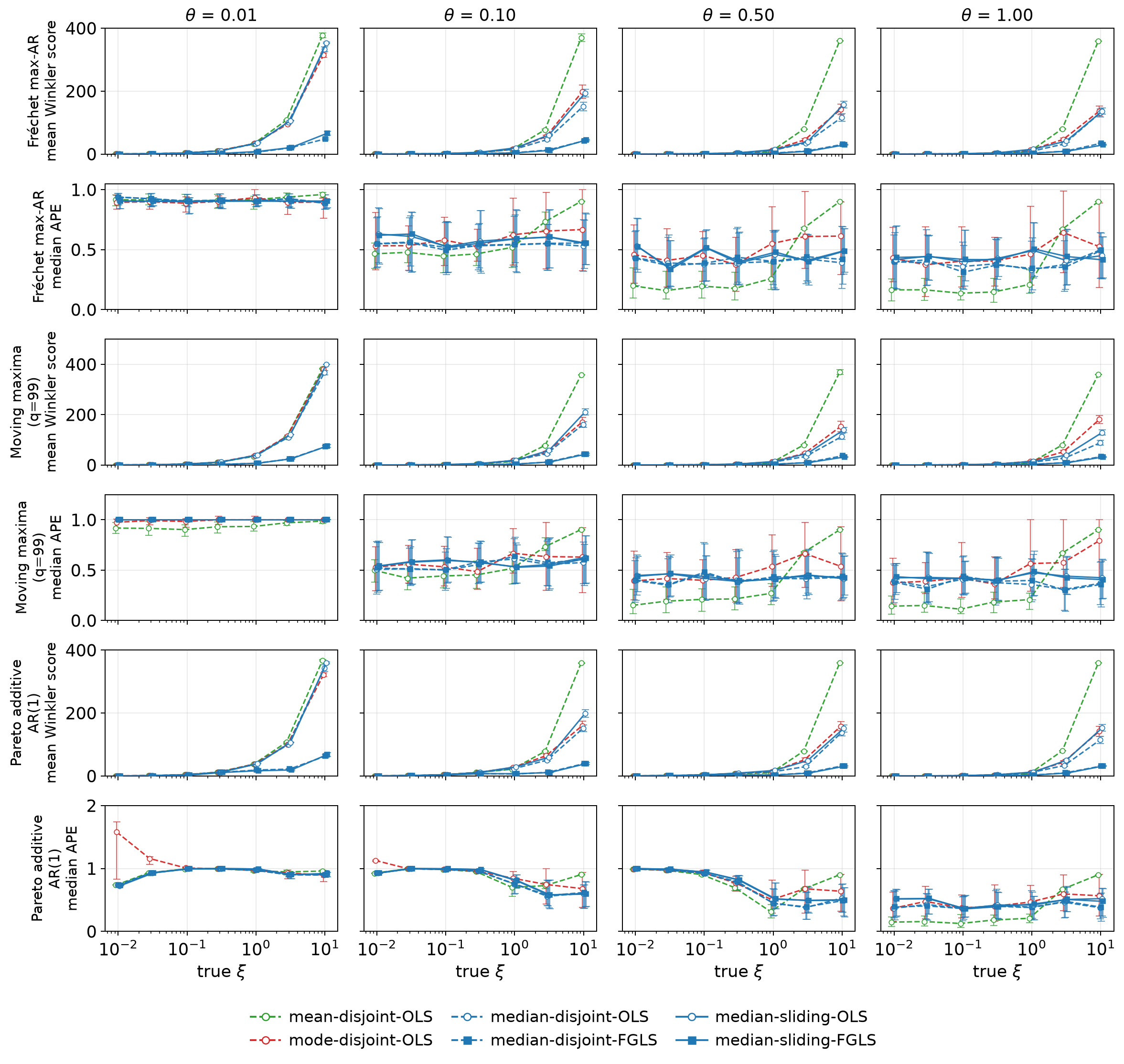
Download all EVI method/scenario summaries (CSV). The external comparison considers seven methods: median-, mean-, and mode-based sliding-FGLS, Hill, max-spectrum, Pickands, and DEdH moment. Within this set, median-sliding-FGLS has the lowest grid-average score and never ranks last in the 84 scenarios. Hill wins 28 scenarios and median-sliding-FGLS wins 14, but their grid-average scores are 25.81 and 9.38, respectively.

Sliding FGLS target	Grid-average Winkler score	Grid-average coverage
Median	9.38	79.0%
Mean	24.94	59.0%
Mode	14.29	76.5%

Hill and max-spectrum have lower grid-average scenario-median APE than these three sliding FGLS methods. This point-error comparison and the interval-score ranking assess different objectives. At xi=0.01, the near-zero denominator can magnify APE. Read coverage and n_score alongside interval scores.

Persistence branch (EI)

The EI suite varies the true extremal index, tail severity, and process family. The chart below compares eight pooled-BM estimators on the dimensionless θ scale.

BB-sliding-FGLS has lower mean Winkler scores than its pooled OLS counterpart in all 84 scenarios. This also holds for each other path/scheme pair. For BB-sliding, the grid-average interval width is 0.1344 under FGLS versus 0.0105 under OLS, and coverage is 47.6% versus 11.9%. Point-error and interval performance remain distinct: the grid-average scenario-median APE is 0.288 under FGLS and 0.271 under OLS.

BB-sliding-FGLS and Northrop-sliding-FGLS have the two lowest within-BM grid-average scores, 1.655 and 1.684, and together win 58 of 84 scenarios. Their grid-average coverages, 47.6% and 48.7%, remain far below 95%.

Eight internal pooled EI methods: BB/Northrop × sliding/disjoint × OLS/FGLS. Mean Winkler score uses ±1 outer MCSE; median absolute percentage error uses its IQR. Click the figure for full size.

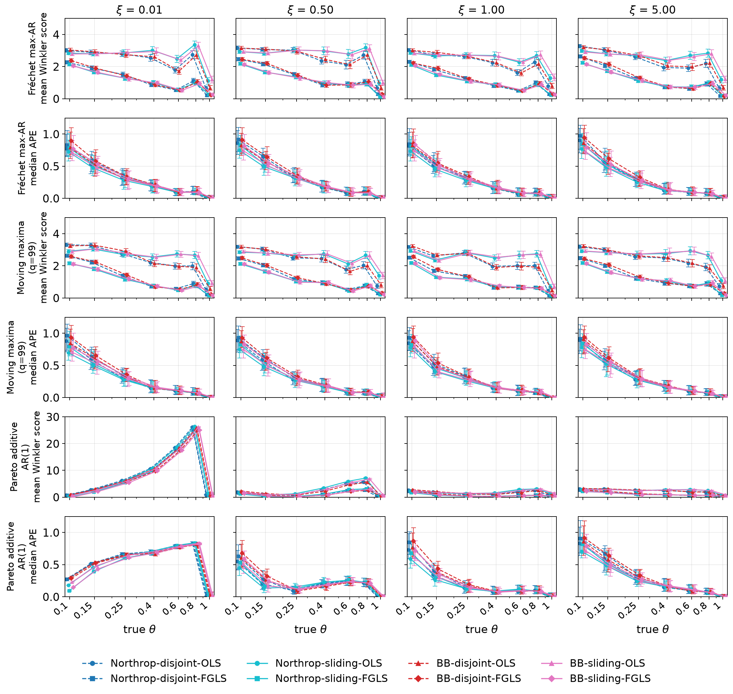
The eight-method external comparison combines the four pooled-BM FGLS variants with Ferro–Segers, K-gaps, native Northrop sliding, and native BB sliding on the same simulated records. BB-sliding-FGLS and native BB are the only methods in this comparison that never rank last by mean Winkler score. BB-sliding-FGLS outperforms native BB in 77 of 84 scenarios, with grid-average scores of 1.655 and 2.106, respectively.

K-gaps has the lowest grid-average score, 1.00, and wins 59 of 84 scenarios. It ranks last in all 12 scenarios with theta=1. These results distinguish BB-sliding-FGLS's consistent within-BM improvement from the advantages of threshold-based estimation in much of the examined grid.

Download all EI method/scenario summaries (CSV). interval_score_mean is the primary score; n_rep counts outer simulated records, not bootstrap R. The grid exhibits substantial undercoverage, so a nominal 95% interval must not be read as having achieved 95% empirical coverage.

Numerical precision and failed fits

An adaptive fit that reaches R=1024 without meeting its numerical precision tolerance is retained and scored, with bootstrap_precision_met=False. This is different from an unusable covariance: strict FGLS does not fall back to OLS. Recorded failed estimates count as misses in coverage and have no finite interval score. The mean score is consequently conditional on valid scored fits; read n_score and failure counts alongside it.

The detailed internal CSVs record actual R, the precision flag, maximum MCSE ratio, and shrinkage. A missing precision flag means it was not assessed for that fit, not that it passed. Adaptive stopping is conditional on the observed fit window and does not establish CI coverage or design-life-level precision.

In this run, 2,433 of 50,400 EVI FGLS fits and 2,364 of 33,573 successful EI FGLS fits reached the cap without meeting the tolerance. Twenty-seven EI FGLS attempts failed because of degenerate covariance (13 BB-sliding and 14 Northrop-sliding, all at true theta=1). The EVI DEdH-moment reference has 421 unscored attempts out of 8,400. These are disclosed separately from adaptive precision-unmet fits.

Changes from the earlier configuration

The comparison below uses the same simulated-record design and seeds as the 2026-09-23 snapshot. It compares the combined changes in block bounds, full-range window selection, EVI super-block handling, and EVI shrinkage; it does not isolate the effect of one setting. The earlier snapshot used lower exponent 0.2, upper exponent 0.55 with at least 15 disjoint blocks, edge trimming, and the EVI 4B rule with segment-count adjustments.

Method	Mean score, earlier → current	Mean coverage, earlier → current	Lower / higher score scenarios
EVI median-sliding-FGLS	9.485 → 9.383	67.3% → 79.0%	39 / 45
EVI median-disjoint-FGLS	10.041 → 9.261	68.2% → 82.3%	55 / 29
EI BB-sliding-FGLS	1.607 → 1.655	50.4% → 47.6%	41 / 43
EI Northrop-sliding-FGLS	1.648 → 1.684	49.5% → 48.7%	42 / 42

Each mean gives equal weight to 84 scenarios; lower score is better. The changes do not improve every scenario or every metric. Both median EVI methods have lower grid-average scores and higher coverage than this earlier snapshot, while the two sliding EI scores and coverages worsen slightly. The grid-average scenario-median APE changes from 0.613 to 0.648 for median-sliding EVI, from 0.268 to 0.288 for BB-sliding EI, and from 0.269 to 0.285 for Northrop-sliding EI. These are descriptive comparisons, not tests of significance or independent validation of the chosen defaults.

Changes from the immediately preceding retained run

The previous retained EVI run used shrinkage 0.37 and no disjoint-block cap. The current rerun restores the n/17 cap and uses shrinkage 0.73, with the same simulated records and seeds. At N=365, the EVI grid changes from 27 levels over 8–41 to 12 levels over 8–21; super-block length changes from 82 to 42. This changes both the candidate windows and the bootstrap construction, so the comparison does not isolate shrinkage or the upper bound.

EVI method	Mean score, preceding → current	Lower / higher score scenarios
Median-disjoint-FGLS	12.010 → 9.261	78 / 6
Median-sliding-FGLS	14.587 → 9.383	72 / 12
Mode-disjoint-FGLS	14.619 → 13.072	69 / 15
Mode-sliding-FGLS	17.751 → 14.295	72 / 12
Mean-disjoint-FGLS	17.371 → 16.934	53 / 31
Mean-sliding-FGLS	38.533 → 24.941	67 / 17

For median-sliding-FGLS, mean width falls from 10.324 to 6.653 and coverage rises from 76.9% to 79.0%. The proportion of estimates with abs(xi_hat) < 1e-10 falls from 60.5% to 11.8%; it is not eliminated. All 50,400 EVI FGLS attempts have finite interval scores. The EI benchmark is numerically unchanged from the immediately preceding run: shrinkage remains 0.37 and the square-root upper bound is active at this record length.

What is and is not validated

Checked here	Boundary
Known-target estimation error and parameter-interval coverage	Only the simulated families, parameter grid, and record length N=365
Error and interval-score comparisons	Finite Monte Carlo design, not an asymptotic proof
Sensitivity to dependence and tail severity	Not robustness to arbitrary nonstationarity or model misspecification
Current fixed-shrinkage/adaptive-R workflow	No claim that data-driven selection uncertainty is fully absorbed
EVI/EI parameter intervals	Coverage of derived design-life intervals has not been evaluated

The case-study pages use archived provider inputs. Eight continuous-record cases use FGLS and adaptive R; the gapped GOES case uses OLS point estimates only. These real-data illustrations have no known true parameters and do not establish coverage of extrapolated physical, monetary, or normalized design-life levels.

Reproduction and scope

The figures and CSVs on this page are retained statistical-validation snapshots. Building the documentation or installing an optimized backend does not regenerate them. They are not runtime benchmarks. To compare execution speed, record the source commit, native/NumPy backend, Python and dependency versions, hardware, thread/process budgets, sample and bootstrap settings, and cache state; verify numerical agreement separately. See execution settings.

To regenerate the full workflow while keeping report exports inside this repository, use:

UNIBM_REPORT_DIR=out/reports just full

This runs the complete tests, clears named generated outputs, recomputes both benchmark grids and shrinkage sensitivity, reruns the six canonical applications, refreshes GOES/SPY/QQQ when their local inputs are available, and builds the documentation. It does not download fresh provider inputs or update hand-written numerical discussion. An explicit UNIBM_REPORT_DIR overrides the local .env destination for this invocation.

After source installation with development dependencies, force the two main grids from the repository root:

UNIBM_FORCE_BENCHMARK=1 just --command uv run python scripts/benchmark/evi_benchmark.py
UNIBM_FORCE_BENCHMARK=1 just --command uv run python scripts/benchmark/ei_benchmark.py

UNIBM_BENCHMARK_WORKERS optionally limits parallel workers. These commands reuse the cached raw simulated records but recompute the estimates. Adaptive fitting bypasses old fixed-R covariance caches. The canonical outputs are out/benchmark/evi_{detail,summary,external_detail,external_summary}.csv and the matching ei_ files. Report functions in scripts/benchmark/evi_report.py and ei_report.py generate the static plots from those summaries.

This page covers the two complete main grids, including their external comparators. Neither a site build nor these two commands downloads provider data or reruns applications.

Shrinkage sensitivity

The shrinkage sensitivity analysis varies delta = 0, 0.15, 0.37, 0.55, 0.75, 1 for EI and additionally 0.73 for EVI, using mean Winkler score as the primary metric. It covers median-sliding-FGLS EVI and BB/Northrop sliding-FGLS EI on the same main grids. Median coverage and median APE remain secondary diagnostics. Family summaries give equal weight to scenario-level mean scores, with no normalization.

For each simulated record, the original selected window and the bootstrap draws obtained by adaptive stopping at the branch default (delta=0.73 for EVI, 0.37 for EI) are reused across the grid. R is not independently retuned at each delta, and the default-fit precision flag does not certify the other delta fits. Failed EI covariances are retained as noncoverage, with no finite score, at every delta.

With the current EVI grid, diagonal shrinkage reduces the grid-average score from 22.138 at delta=0 to 9.383 at the default 0.73. The default has the lowest score among the seven tested values; 0.75 gives 9.388 and full diagonal shrinkage gives 9.599. This identifies a minimum on this retained grid, not a universal optimum or an independent validation of the default.

The EI scores are 1.655 (BB) and 1.684 (Northrop) at the default, with minima of 1.635 and 1.656 at 0.15. Full diagonal shrinkage worsens these scores to 2.198 and 2.219 and reduces median coverage. These comparisons do not establish nominal coverage. No additional multiplicative CI calibration is applied.

The existing report entrypoints generate the supplementary CSVs when absent and refresh the report figures:

just --command uv run python scripts/benchmark/evi_report.py
just --command uv run python scripts/benchmark/ei_report.py

The corresponding build_evi_shrinkage_sensitivity_summary and build_ei_shrinkage_sensitivity_summary functions accept force=True to recompute an existing sensitivity CSV. Both accept max_workers; otherwise they use UNIBM_BENCHMARK_WORKERS, including the worker count passed to just benchmark or just reports. Scenarios run in separate processes with unchanged scenario seeds; max_workers=1 runs serially. Adaptive EI sensitivity computes only the requested paths (the two sliding paths by default). Outputs remain under out/benchmark/; no separate validation suite or intermediate storage format is introduced.